안녕하세요.
오늘의 파이썬 코딩 독학 주제는 Matplotlib 입니다.
1. Matplotlib란?
파이썬에서 데이터를 시각화하도록 도와주는 패키지입니다.
그래프를 그려주고, 차트를 만들어주는 등 다양한 기능을 제공하여
다양한 방면으로 사용되고 있습니다.
2. 필요한 라이브러리
이번 예제를 다루기 위해서는 두가지 라이브러리가 추가로 필요합니다.
다음 명령어를 이용하여 라이브러리를 다운받아주세요.
pip install matplotlib
pip install numpy
3. 전체 소스코드
import tensorflow as tf
import matplotlib.pyplot as plt
import numpy as np

from tensorflow.examples.tutorials.mnist import input_data
mnist = input_data.read_data_sets("./mnist/data/", one_hot=True)

keep_prob = tf.placeholder(tf.float32)

X = tf.placeholder(tf.float32, [None, 784])
Y = tf.placeholder(tf.float32, [None, 10])

W1 = tf.Variable(tf.random_normal([784, 256], stddev=0.01))
L1 = tf.nn.relu(tf.matmul(X, W1))
L1 = tf.nn.dropout(L1, 0.8)

W2 = tf.Variable(tf.random_normal([256, 256], stddev=0.01))
L2 = tf.nn.relu(tf.matmul(L1, W2))
L2 = tf.nn.dropout(L2, 0.8)

W3 = tf.Variable(tf.random_normal([256, 10], stddev=0.01))
model = tf.matmul(L2, W3)

cost = tf.reduce_mean(tf.nn.softmax_cross_entropy_with_logits_v2(logits=model, labels=Y))
optimizer = tf.train.AdamOptimizer(0.001).minimize(cost)

init = tf.global_variables_initializer()
sess = tf.Session()
sess.run(init)

batch_size = 100
total_batch = int(mnist.train.num_examples / batch_size)

for epoch in range(30):
    total_cost = 0

    for i in range(total_batch):
        batch_xs, batch_ys = mnist.train.next_batch(batch_size)

        _, cost_val = sess.run([optimizer, cost], feed_dict = {X:batch_xs, Y:batch_ys, keep_prob: 0.8})

        total_cost += cost_val

    print('Epoch:', '%04d' % (epoch + 1), 'Avg. cost=', '{:.3f}'.format(total_cost / total_batch))

print('최적화 완료')

is_correct = tf.equal(tf.argmax(model, 1), tf.argmax(Y, 1))

accuracy = tf.reduce_mean(tf.cast(is_correct, tf.float32))

print('정확도:', sess.run(accuracy, feed_dict={X: mnist.test.images, Y: mnist.test.labels, keep_prob: 1}))

labels = sess.run(model, feed_dict={X: mnist.test.images, Y: mnist.test.labels, keep_prob: 1})

fig = plt.figure()
for i in range(10):
    subplot = fig.add_subplot(2, 5, i + 1)
    subplot.set_xticks([])
    subplot.set_yticks([])
    subplot.set_title('%d' % np.argmax(labels[i]))
    subplot.imshow(mnist.test.images[i].reshape((28, 28)), cmap = plt.cm.gray_r)

plt.show()
4. 소스코드의 목적
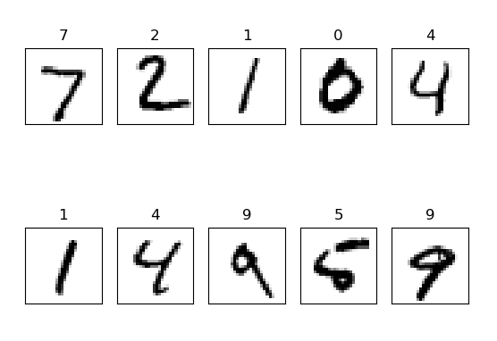
지난시간에 배운 MNIST코드를 활용하여 분석결과를 그림으로 표현하기 위한 코드입니다.
분석한 손글씨와, 예측값을 대조한 그래프를 화면에 표시해보겠습니다.
5. 소스코드 분석
우선 라이브러리를 추가하겠습니다.
import matplotlib.pyplot as plt
import numpy as np
이번엔 테스트 데이터를 활용해 학습을 진행하고, 결과값을 labels라는 변수에 저장하겠습니다.
labels = sess.run(model, feed_dict={X: mnist.test.images, Y: mnist.test.labels, keep_prob: 1})
다음으로는 출력을 위한 그래프를 세팅하고,
테스트 데이터의 1~10번째 이미지와 그에 대한 예측값을 출력하도록 하겠습니다.
fig = plt.figure()

for i in range(10):
    subplot = fig.add_subplot(2, 5, i + 1)
    subplot.set_xticks([])
    subplot.set_yticks([])
    subplot.set_title('%d' % np.argmax(labels[i]))
    subplot.imshow(mnist.test.images[i].reshape((28, 28)), cmap = plt.cm.gray_r)

plt.show()
여기서 plt.figure()함수와
fig.add_subplot(행, 열, 숫자 이미지 출력할 순서)함수,
subplot.set_xticks([눈금])함수,
subplot.set_yticks([눈금])함수로 그래프를 세팅합니다.
이번에는 눈금을 출력하지 않고 그래프를 생성하려 하니 눈금란은 비워주세요.
이제 세부설정을 해보겠습니다.
subplot.set_title('%d' % np.argmax(labels[i]))함수를 활용하여
출력할 이미지 위에 예측한 숫자를 출력합니다.
이때 np.argmax()함수는 tf.argmax()함수와 동일한 기능을 합니다.
결과값인 labels의 i번째 요소가 원-핫 인코딩 형식이므로
해당배열에서 가장 높은 값을 가진 인덱스를 예측한 숫자로 반환합니다.
subplot.imshow(mnist.test.images[i].reshape((28, 28)), cmap = plt.cm.gray_r)함수를 활용하여
1차원 배열로 되어있는 i번째 이미지 데이터를
28x28 형식의 2차원 배열로 변형하여 이미지 형태로 출력하고,
cmap 파라미터를 통해 이미지를 그레이 스케일로 출력합니다.
plt.show() 함수를 이용해 그래프를 화면에 표시합니다.
6. 결과 확인
무사히 잘 따라오셨다면 다음과 같은 그림이 출력됩니다.
'코딩 > 텐서플로우' 카테고리의 다른 글
| 비전공자의 코딩 독학 - 파이썬&텐서플로우(14) <오토인코더> (0) | 2020.05.04 |
|---|---|
| 비전공자의 코딩 독학 - 파이썬&텐서플로우(13) <CNN> (0) | 2020.05.03 |
| 비전공자의 코딩 독학 - 파이썬&텐서플로우(11) <과적합> (0) | 2020.04.30 |
| 비전공자의 코딩 독학 - 파이썬&텐서플로우(10) <MNIST> (0) | 2020.03.11 |
| 비전공자의 코딩 독학 - 파이썬&텐서플로우(9) <시그모이드 예제> (0) | 2020.01.18 |


